In the previous post, we gave you some insights about the simulation of simple birth-death processes with simmer. The extension of such a methodology for more complex queueing networks is immediate and was left as an exercise for the reader.
Similarly, today we are going to explore more features of simmer with a simple Continuous-Time Markov Chain (CTMC) problem as an excuse. CTMCs are more general than birth-death processes (those are special cases of CTMCs) and may push the limits of our simulator. So let’s start.
A gas station has a single pump and no space for vehicles to wait (if a vehicle arrives and the pump is not available, it leaves). Vehicles arrive to the gas station following a Poisson process with a rate of 


This problem is described by the following CTMC:
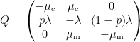
with 

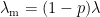
with the constraint

There are 
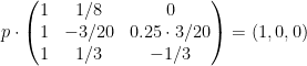
The solution 

# Arrival rate
lambda <- 3/20
# Service rate (cars, motorcycles)
mu <- c(1/8, 1/3)
# Probability of car
p <- 0.75

# Theoretical resolution
A <- matrix(c(1,   mu[1],            0,
              1, -lambda, (1-p)*lambda,
              1,   mu[2],       -mu[2]), byrow=T, ncol=3)
B <- c(1, 0, 0)
P <- solve(t(A), B)
N_average_theor <- sum(P * c(1, 0, 1)) ; N_average_theor
## [1] 0.5031056Now, we are going to simulate the system with simmer and verify that it converges to the theoretical solution. There are various options for selecting the model. As a first approach, due to the properties of Poisson processes, we can break down the problem into two trajectories (one for each type of vehicle), which differ in their service time only, and therefore two generators with rates 
library(simmer)
set.seed(1234)

option.1 <- function(t) {
  car <- create_trajectory() %>%
    seize("pump", amount=1) %>%
    timeout(function() rexp(1, mu[1])) %>%
    release("pump", amount=1)

  mcycle <- create_trajectory() %>%
    seize("pump", amount=1) %>%
    timeout(function() rexp(1, mu[2])) %>%
    release("pump", amount=1)

  simmer() %>%
    add_resource("pump", capacity=1, queue_size=0) %>%
    add_generator("car", car, function() rexp(1, p*lambda)) %>%
    add_generator("mcycle", mcycle, function() rexp(1, (1-p)*lambda)) %>%
    run(until=t)
}
Other arrival processes may not have this property, so we would define a single generator for all kind of vehicles and a single trajectory as follows. In order to distinguish between cars and motorcycles, we could define a branch after seizing the resource to select the proper service time.
option.2 <- function(t) {
  vehicle <- create_trajectory() %>%
    seize("pump", amount=1) %>%
    branch(function() sample(c(1, 2), 1, prob=c(p, 1-p)), continue=c(T, T),
           create_trajectory("car") %>%
             timeout(function() rexp(1, mu[1])),
           create_trajectory("mcycle") %>%
             timeout(function() rexp(1, mu[2]))) %>%
    release("pump", amount=1)

  simmer() %>%
    add_resource("pump", capacity=1, queue_size=0) %>%
    add_generator("vehicle", vehicle, function() rexp(1, lambda)) %>%
    run(until=t)
}
But this option adds an unnecessary overhead since there is an additional call to an R function to select the branch, and therefore performance decreases. A much better option is to select the service time directly inside the timeout function.
option.3 <- function(t) {
  vehicle <- create_trajectory() %>%
    seize("pump", amount=1) %>%
    timeout(function() {
      if (runif(1) < p) rexp(1, mu[1])  # car
      else rexp(1, mu[2])               # mcycle
    }) %>%
    release("pump", amount=1)

  simmer() %>%
    add_resource("pump", capacity=1, queue_size=0) %>%
    add_generator("vehicle", vehicle, function() rexp(1, lambda)) %>%
    run(until=t)
}
This option.3 is equivalent to option.1 in terms of performance. But, of course, the three of them lead us to the same result. For instance,
gas.station <- option.3(5000)

library(ggplot2)

# Evolution + theoretical value
graph <- plot_resource_usage(gas.station, "pump", items="system")
graph + geom_hline(yintercept=N_average_theor)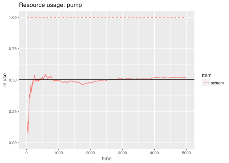
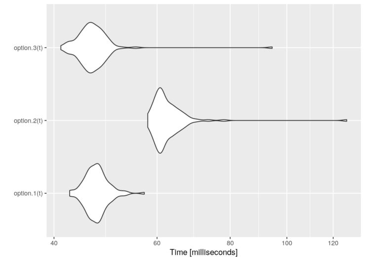
And these are some performance results:
library(microbenchmark)

t <- 1000/lambda
tm <- microbenchmark(option.1(t),
                     option.2(t),
                     option.3(t))
graph <- autoplot(tm)
graph + scale_y_log10(breaks=function(limits) pretty(limits, 5)) +
  ylab("Time [milliseconds]")