Simulating queueing systems with ‘simmer’

The M/M/1 system

In Kendall’s notation, an M/M/1 system has exponential arrivals (M/M/1), a single server (M/M/1) with exponential service time (M/M/1) and an inifinite queue (implicit M/M/1/). For instance, people arriving at an ATM at rate , waiting their turn in the street and withdrawing money at rate .

Let us remember the basic parameters of this system:

whenever . If that is not true, it means that the system is unstable: there are more arrivals than the server is capable of handling, and the queue will grow indefinitely.

The simulation of an M/M/1 system is quite simple using simmer. The trajectory-based design, combined with magrittr’s pipe, is very verbal and self-explanatory.

library(simmer)
set.seed(1234)

lambda <- 2
mu <- 4
rho <- lambda/mu # = 2/4

mm1.trajectory <- create_trajectory() %>%
  seize("resource", amount=1) %>%
  timeout(function() rexp(1, mu)) %>%
  release("resource", amount=1)

mm1.env <- simmer() %>%
  add_resource("resource", capacity=1, queue_size=Inf) %>%
  add_generator("arrival", mm1.trajectory, function() rexp(1, lambda)) %>% 
  run(until=2000)

Our package provides convenience plotting functions to quickly visualise the usage of a resource over time, for instance. Down below, we can see how the simulation converges to the theoretical average number of customers in the system.

library(ggplot2)

# Evolution of the average number of customers in the system
graph <- plot_resource_usage(mm1.env, "resource", items="system")

# Theoretical value
mm1.N <- rho/(1-rho)
graph + geom_hline(yintercept=mm1.N)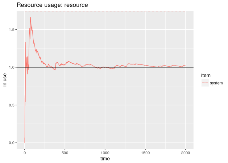

It is possible also to visualise, for instance, the instantaneous usage of individual elements by playing with the parametersitems and steps.

plot_resource_usage(mm1.env, "resource", items=c("queue", "server"), steps=TRUE) +
  xlim(0, 20) + ylim(0, 4)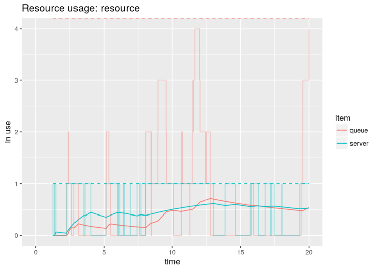

We may obtain the time spent by each customer in the system and we compare the average with the theoretical expression.

mm1.arrivals <- get_mon_arrivals(mm1.env)
mm1.t_system <- mm1.arrivals$end_time - mm1.arrivals$start_time

mm1.T <- mm1.N / lambda
mm1.T ; mean(mm1.t_system)

## [1] 0.5

## [1] 0.5012594

It seems that it matches the theoretical value pretty well. But of course we are picky, so let’s take a closer look, just to be sure (and to learn more about simmer, why not). Replication can be done with standard R tools:

library(parallel)

envs <- mclapply(1:1000, function(i) {
  simmer() %>%
    add_resource("resource", capacity=1, queue_size=Inf) %>%
    add_generator("arrival", mm1.trajectory, function() rexp(1, lambda)) %>%
    run(1000/lambda) %>%
    wrap()
})

Et voilà! Parallelizing has the shortcoming that we lose the underlying C++ objects when each thread finishes, but the wrapfunction does all the magic for us retrieving the monitored data. Let’s perform a simple test:

library(dplyr)

t_system <- get_mon_arrivals(envs) %>%
  mutate(t_system = end_time - start_time) %>%
  group_by(replication) %>%
  summarise(mean = mean(t_system))

t.test(t_system$mean)

## 
##  One Sample t-test
## 
## data:  t_system$mean
## t = 348.23, df = 999, p-value < 2.2e-16
## alternative hypothesis: true mean is not equal to 0
## 95 percent confidence interval:
##  0.4957328 0.5013516
## sample estimates:
## mean of x 
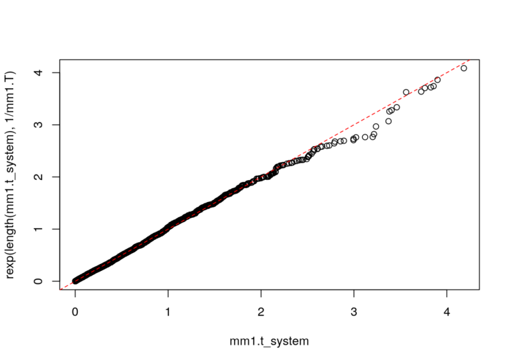
## 0.4985422

Good news: the simulator works. Finally, an M/M/1 satisfies that the distribution of the time spent in the system is, in turn, an exponential random variable with average .

qqplot(mm1.t_system, rexp(length(mm1.t_system), 1/mm1.T))
abline(0, 1, lty=2, col="red")

 

M/M/c/k systems

An M/M/c/k system keeps exponential arrivals and service times, but has more than one server in general and a finite queue, which often is more realistic. For instance, a router may have several processor to handle packets, and the in/out queues are necessarily finite.

This is the simulation of an M/M/2/3 system (2 server, 1 position in queue). Note that the trajectory is identical to the M/M/1 case.

lambda <- 2
mu <- 4

mm23.trajectory <- create_trajectory() %>%
  seize("server", amount=1) %>%
  timeout(function() rexp(1, mu)) %>%
  release("server", amount=1)

mm23.env <- simmer() %>%
  add_resource("server", capacity=2, queue_size=1) %>%
  add_generator("arrival", mm23.trajectory, function() rexp(1, lambda)) %>%
  run(until=2000)

In this case, there are rejections when the queue is full.

mm23.arrivals <- get_mon_arrivals(mm23.env)
mm23.arrivals %>%
  summarise(rejection_rate = sum(!finished)/length(finished))

##   rejection_rate
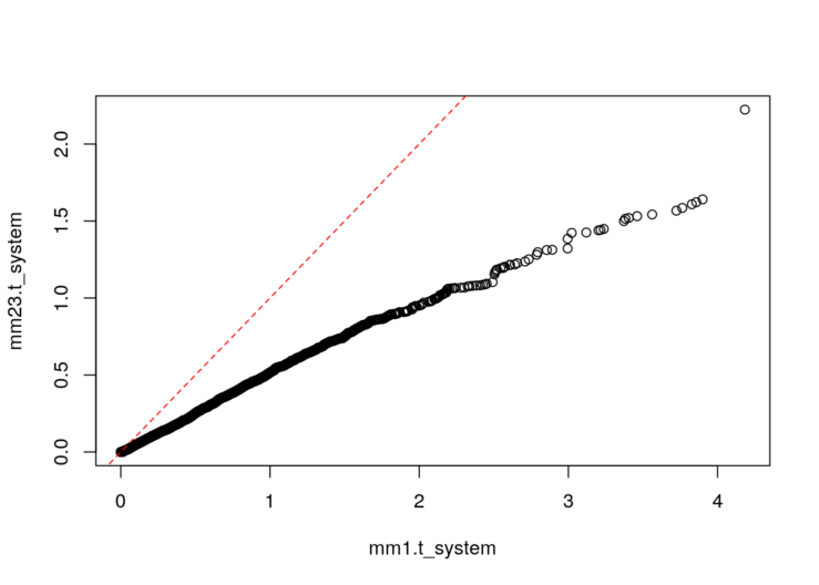
## 1     0.02009804

Despite this, the time spent in the system still follows an exponential random variable, as in the M/M/1 case, but the average has dropped.

mm23.t_system <- mm23.arrivals$end_time - mm23.arrivals$start_time
# Comparison with M/M/1 times
qqplot(mm1.t_system, mm23.t_system)
abline(0, 1, lty=2, col="red")